Harnessing artificial intelligence for environmental sustainability via human capital and renewable energy

Theoretical framework

The impact of artificial intelligence (AI) on CO2 emissions is determined through “technological innovation theory”, which postulates that an increase in emerging technologies can drive environmental quality by increasing energy efficiency and reducing the use of dirty and traditional technologies. From the seminal work of (Lundvall, 1992) on the use of technologies in sustainability⁴³, technologies and the application of human learning through technologies such as artificial intelligence. In addition, AI can help address climate change with indispensable efforts (i.e., from tracking melting icebergs to mapping deforested areas to recycling items that would not have been possible before) around the world. With all its possibilities, AI can have a negative impact on climate change and environmental sustainability. The increase in AI leads to more electronic waste and more data storage, which creates a material footprint for storing and cooling the available data. Hence, given the positive impact of AI on CO2 emissions, we hypothesize that AI will have an adverse effect on our diverse sample of countries that have adopted AI systems, i.e., mathematically represented as \(\:{\alpha\:}^{1}\:=\partial\:{{CO2}_{it}/AIPTNTS\partial\:}_{it}\:>0\). However, in terms of the negative effect of AI and providing support for the reduction of environmental degradation, we expect a negative influence, i.e., \(\:{\alpha\:}^{1}\:=\partial\:{{CO2}_{it}/AIPTNTS\partial\:}_{it}\:<0\).

In addition, the use of technologies such as renewable energy technologies and their consumption can reduce carbon emissions because of their replacement with energy generated from dirty sources (i.e., fossil fuels). Renewable energy consumption can be channeled toward the environment through energy transition theory^44,45,46, which postulates that shifting from dirty sources of energy and fossil fuels to cleaner energy, such as renewable energy (solar and wind), can reduce carbon emissions significantly because of its self-replenished qualities and zero emissions in the environment. Moreover, renewable energy is efficient and can increase sustainable development and the environment. To efficiently transform into cleaner energy, we expect a large reduction in CO2 emissions, which is expressed as \(\:{\alpha\:}^{2}\:=\partial\:{{CO2}_{it}/RECN\partial\:}_{it}\:<0\). The relationship may be positive if the consumption of energy or its proportion is not high enough for renewable energy, i.e., \(\:{\alpha\:}^{3}\:=\partial\:{{CO2}_{it}/RECN\partial\:}_{it}\:>0\).

Moreover, the assimilation of AI and clean energy systems, specifically renewable energy systems, has revolutionized industries by maintaining sustainable economic growth without harming the environment. Theoretically, this underscores the idea of sustainable development, which strives for the enhancement of technologies and innovation and creates harmony between economic expansion and the environment. The use of innovative technologies and applications related to AI helps in the prediction, monitoring, detection and control of energy grids and their solutions. Furthermore, AI enhances real-time monitoring, which further enhances the efficiency of operations, and fault detection, which causes a reduction in intermittence and reliability issues in renewable energy while amplifying its effect on reducing CO2 emissions. Such joint technological innovation directs environmental improvements and amplifies their ability to reduce GHG emissions. Hence, AI promotes the environment by intelligently monitoring energy management and its reliability, while clean energy replaces fossil fuels to target CO2 emissions independently. However, their interaction enhances the reliability, scalability and responsiveness of clean energy products, maximizing their carbon abatement potential. Henceforth, we hypothesize that the moderate effect of AI and clean energy causes a reduction in CO2 emissions. \(\:{\alpha\:}^{4}\:=\partial\:{{CO2}_{it}/\text{A}\text{I}RELTP\partial\:}_{it}\:>0\).

Similarly, renewable electricity has a significant relationship with carbon emissions. By channeling its impact toward a sustainable environment, it is believed that decarbonization theory supports the argument that generating electricity from solar energy and wind reduces CO2 emissions because these energy generation sources do not produce CO2 emissions when generating electricity. The idea is that increasing the share of renewable electricity in the energy mix will lessen carbon intensity and promote a sustainable environment. Hence, we hypothesize a greater share of renewable electricity in the energy mix and therefore expect a reduction in CO2 emissions, which can be represented as \(\:{\alpha\:}^{3}\:=\partial\:{{CO2}_{it}/RECN}_{it}\:>0\). Moreover, we believe that renewable electricity production can strengthen the impact of and relationship between AI and CO2 emissions in our sample countries. Producing renewable electricity and mapping its generation more efficiently through AI can further increase environmental quality.

In addition to the energy perspective, strong human capital (HCI) and development can support activities toward the environment by reducing CO2 emissions. The impact of HCIs is channeled through CO2 emissions through endogenous growth theory⁴⁷. The theory assumes that growth is dependent on internal factors rather than external factors, which is expanded to the environmental perspective by stating that increasing skilled human capital will opt more for efficient and energy-cost-saving models to reduce pollution and waste while enhancing environmental quality. A strongly educated workforce ensures high levels of technological innovation and conducts R&D activities, which reduces the efficiency of output and decreases CO2 emissions. For this purpose, we hypothesize that HCIs strongly support environmental quality by reducing CO2 emissions, i.e., \(\:{\alpha\:}^{6}\:=\partial\:{{CO2}_{it}/HCI\partial\:}_{it}\:>0\). Figure 3 provides a flowchart for the general model specification:

Data and methodology

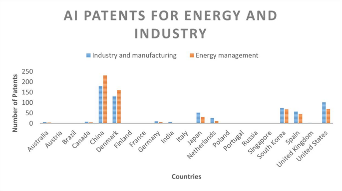
For carbon emissions (CO2 emissions), renewable energy consumption and renewable electricity output data are sourced from the World Bank (2023), World Development Indicators (WDI). For artificial intelligence, we collected the data of the AIPTNTS from the International Federation of Robotics (IFR), 2023, and (OurWorldInData.org,2 023), whereas the data for the human capital index were sourced from International Monetary Fund (IMF), 2023, https://data.imf.org/⁴⁸. Moreover, we utilize a panel dataset ranging from 2010 to 2020 (due to non-availability of data, the time period is from 2010 to 2020), and the countries included in the panel include Australia, Austria, Brazil, Canada, China, Denmark, Finland, France, Germany, India, Italy, Japan, the Netherlands, Poland, Portugal, Russia, Singapore, South Korea, Spain, the United Kingdom, and the United States.

The hypothesized variables of our study are presented in regression models from 1 to 3 in the following equations:

In Eqs. 1, 2 and 3, CO2 emissions are the dependent variable, which represents CO2 emissions in kilotons, whereas the right side represents the independent and control variables, which are further explained with their units of measurement in Table A1 in Appendix A.

Estimation techniques

Descriptive statistics and normality of the data

The data estimation and analysis begin with a general description of the data in a precise manner. Descriptive statistics include average values of the variables, medians, and ranges, which consist of minimum and maximum values. Similarly, the dispersion and volatility of the data are measured through standard deviation (SD) values. In addition, skewness and kurtosis are given, which provide the distributions of the data values, and their threshold levels are defined as 1 and 3, respectively. For a comprehensive examination of the normality of the data, we also employed Jarque-Bera (1987). This test checks the normality of the data and determines whether the data are normally distributed. The following equation is provided for the JB test:

When the values obtained from the JB test are found to be significant, the data are considered nonnormally distributed.

Unit root testing

Prior to explaining the unit root, we first check for cross-sectional dependency (CD) and slope homogeneity (SH) issues in the panel data. Notably, the identification of CD and SH issues is important for determining and employing correct unit root tests (URTs). These URTs include 1^st−, 2^nd− and 3rd -generation tests that target and resolve these issues⁵⁰. To understand the cross-sectional dependency (CD) issue, countries are expected to share different traits, be somewhat dependent on each other and share similar qualities; hence, ignoring this issue and taking panel data cross-sectionally independently will create spurious regression and result in incorrect specifications of unit root tests and cointegration^51,52. Hence, to properly resolve this issue, we employed the CD diagnostic test developed by⁵³. Another issue that should be diagnosed before employing the unit root is the slope homogeneity issue in panel data. Countries with different characteristics can show homogeneity in the data, such as consistent effects of variables across countries, which poses a problem for panel data estimation. To address the homogenizing effects across countries, we employ the⁵⁴ slope heterogeneity test to avoid distorted and biased outcomes. The equation for the SH test is as follows:

In the equations above, \(\:\varDelta\:{\sim}_{SH}\) and \(\:\varDelta\:{\sim}_{ASH}\) are the delta tide and adjusted delta tide, respectively, whereas the statistics S, R and I are from the Swamy test, which is rephrased in the current test⁵⁴. These terms are t-statistics predictors and cross-sectional limits.

After examining the CD and SH issues and confirming their presence, we use both 1st and 2nd-generation panel unit root tests to fully investigate and incorporate variable stationarity in the presence of CD and SH and to reduce the number of distortions in the data. The 1 st generation unit root test includes^55,57 and⁵⁶ and (IPS,2003; Choi, 2001)⁵⁸ and⁵⁹. The first two tests of the 1 st generation are common, whereas the latter two tests are individual URT tests. These approaches are straightforward and can be used in most panel empirical settings⁶⁰. However, the second-generation panel URT is better equipped for dealing with CD and SH issues in the data. Henceforth, we incorporated both tests to efficiently obtain the URT estimations without any biased or distorted outcomes. The cross-sectional augmented Im–Persaran–Shin (CIPS) unit test proposed by⁶¹ offers more robust and consistent outcomes of panel URT. To determine the integrating characteristics of variables, we explore this method in the presence of CD and SH issues. The provision of test statistics is ensured through a cross-sectionally augmented Dickey fuller (CADF) CIPS unit root test. The test statistics of CADF are as follows:

where \(\:{y}_{t}\) in the above equation is the cross-sectional average, and the CIPS equation is given as:

For the nonparametric approach, the integration order should be the first difference.

Cointegration testing

The integration of the variables allows us to determine the cointegration of these variables. The cointegration approach is necessary before we use our primary and main methods for the study. Second-generation panel unit root tests, such as the Kao (1999) cointegration test, address cross-sectional dependency and slope heterogeneity issues. Moreover, the Kao test ensures and addresses every point of the panel data variables and their long-term equilibrium. When no cointegration is found or exists in the variables, its null hypothesis remains stable, whereas the alternative hypothesis is for long-run cointegration among variables.

Primary analysis

When the panel data have outcomes related to unit root and cointegration, the primary method we use in this study is the method of moments of quantile regression (MMQR)⁶² introduced by⁶³. This model can accurately capture the distributional heterogeneity of artificial intelligence and the environment. Moreover, it is more advanced and robust than the simple quantile regression introduced earlier by⁶⁴. Moreover, the research objectives and data specifications can be more properly followed through this model. Notably, the MMQR is more robust for the following reasons, which allows us to implement this model. First, it offers more valid results when the data have no linearity in terms of the parameters and when the data are nonnormally distributed. Second, the MMQR allows different variables to be taken and the issue of uneven distribution to be resolved. Third, the MMQR measures the scale and location of the variables according to their distribution and provides an understanding of how much they tend to differ from the center values⁶⁵. Fourth, the MMQR is valid and robust to outliers and can handle heterogeneity across factors for dependent variables⁶⁶. The following equation specifies the condition quantile location and scale, i.e.,

In this equation, \(\:{\gamma\:}_{i}and\:{\sigma\:}_{i}\) can be termed fixed effects, while the coefficients in this equation are \(\:\gamma\:\), \(\:\phi\:\:,\sigma\:\) and \(\:\alpha\:\). However, its probability equation is \(\:P\:\left({\sigma\:}_{i}+\phi\:.\:{X}_{it}>0\right)=1.\), where the K vector is represented through R and denoted by X as:

Furthermore, \(\:{R}_{it}\) in the equation follows the uniform approach across “i” and “t”. Similarly, it will remain unaffected and orthogonal to the external factors across the model by reducing its influence. Consequently, the MMQR model is presented in the subsequent equation created from the above equations, i.e.,

In this equation, \(\:{R}_{it}\) expresses exogenous variables, and \(\:{H}_{it}\) represents the dependent variable, i.e., environmental sustainability. Moreover, the final model presented for our study without our variables included \(\:q\left(\tau\:\right)\), which represents different sets of quantiles. Hence, the final equation is given below:

Dumitrescu and Hurlin (2012) panel causality test

To better examine and incorporate cross-sectional dependency and slope heterogeneity, we employ the Dumitrescu and Hurlin (D-H) (2012) panel causality test related to time series Granger causality⁶⁷. The DH test uses a linear model, which is given below:

where “i” and “t” are the cross sections and time, respectively, while \(\:{\alpha\:}_{i}\) and \(\:{\beta\:}_{i}\) are the slope and coefficients, respectively, and where \(\:{\gamma\:}_{i}^{\left(K\right)}\) and \(\:{\beta\:}_{i}^{\left(K\right)}\) are the autoregressive parameters. The DH causality tests keep the null hypothesis as no causal relationship between variables.